首页 - 互联网

Python机器学习笔记：XgBoost算法

作者: 五速梦信息网
时间: 2026年04月04日 13:32

前言

1，Xgboost简介

　　Xgboost是Boosting算法的其中一种，Boosting算法的思想是将许多弱分类器集成在一起，形成一个强分类器。因为Xgboost是一种提升树模型，所以它是将许多树模型集成在一起，形成一个很强的分类器。而所用到的树模型则是CART回归树模型。

　　Xgboost是在GBDT的基础上进行改进，使之更强大，适用于更大范围。

　　Xgboost一般和sklearn一起使用，但是由于sklearn中没有集成Xgboost，所以才需要单独下载安装。

2，Xgboost的优点

　　Xgboost算法可以给预测模型带来能力的提升。当我们对其表现有更多了解的时候，我们会发现他有如下优势：

2.1 正则化

　　实际上，Xgboost是以“正则化提升（regularized boosting）” 技术而闻名。Xgboost在代价函数里加入了正则项，用于控制模型的复杂度。正则项里包含了树的叶子节点个数，每个叶子节点上输出的score的L2模的平方和。从Bias-variance tradeoff角度来讲，正则项降低了模型的variance，使学习出来的模型更加简单，防止过拟合，这也是Xgboost优于传统GBDT的一个特征

2.2 并行处理

　　Xgboost工具支持并行。众所周知，Boosting算法是顺序处理的，也是说Boosting不是一种串行的结构吗？怎么并行的？注意Xgboost的并行不是tree粒度的并行。Xgboost也是一次迭代完才能进行下一次迭代的（第t次迭代的代价函数里包含）。Xgboost的并行式在特征粒度上的，也就是说每一颗树的构造都依赖于前一颗树。

　　我们知道，决策树的学习最耗时的一个步骤就是对特征的值进行排序（因为要确定最佳分割点），Xgboost在训练之前，预先对数据进行了排序，然后保存为block结构，后面的迭代中重复使用这个结构，大大减小计算量。这个block结构也使得并行成为了可能，在进行节点的分类时，需要计算每个特征的增益，大大减少计算量。这个block结构也使得并行成为了可能，在进行节点的分裂的时候，需要计算每个特征的增益，最终选增益最大的那个特征去做分裂，那么各个特征的增益计算就可以开多线程进行。

2.3 灵活性

　　Xgboost支持用户自定义目标函数和评估函数，只要目标函数二阶可导就行。它对模型增加了一个全新的维度，所以我们的处理不会受到任何限制。

2.4 缺失值处理

　　对于特征的值有缺失的样本，Xgboost可以自动学习出他的分裂方向。Xgboost内置处理缺失值的规则。用户需要提供一个和其他样本不同的值，然后把它作为一个参数穿进去，以此来作为缺失值的取值。Xgboost在不同节点遇到缺失值时采用不同的处理方法，并且会学习未来遇到缺失值时的处理方法。

2.5 剪枝

　　Xgboost先从顶到底建立所有可以建立的子树，再从底到顶反向机芯剪枝，比起GBM，这样不容易陷入局部最优解

2.6 内置交叉验证

　　Xgboost允许在每一轮Boosting迭代中使用交叉验证。因此可以方便的获得最优Boosting迭代次数，而GBM使用网格搜索，只能检测有限个值。

3，Xgboost的离线安装

1，点击此处，下载对应自己Python版本的网址。

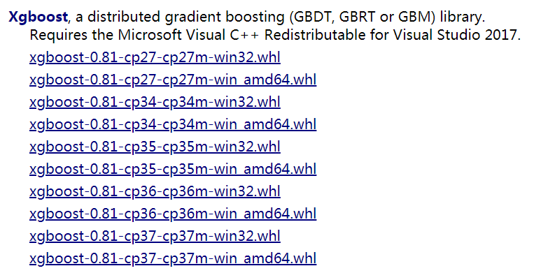
2，输入安装的程式：

pip install xgboost-0.81-cp37-cp37m-win_amd64.whl

Xgboost模型详解

1，Xgboost能加载的各种数据格式解析

　　Xgboost可以加载多种数据格式的训练数据：

libsvm 格式的文本数据；
Numpy 的二维数组；
XGBoost 的二进制的缓存文件。加载的数据存储在对象 DMatrix 中。

　　　下面一一列举：

　　记载libsvm格式的数据

dtrain1 = xgb.DMatrix('train.svm.txt')

　　记载二进制的缓存文件

dtrain2  = xgb.DMatrix('train.svm.buffer')

　　加载numpy的数组

data = np.random.rand(5,10)                 # 5行10列数据集

label = np.random.randint(2,size=5)       # 二分类目标值

dtrain = xgb.DMatrix(data,label=label)    # 组成训练集

　　将scipy.sparse格式的数据转化为Dmatrix格式

csr = scipy.sparse.csr_matrix((dat,(row,col)))

dtrain = xgb.DMatrix( csr )

　　将Dmatrix格式的数据保存成Xgboost的二进制格式，在下次加载时可以提高加载速度，使用方法如下：

dtrain = xgb.DMatrix('train.svm.txt')

dtrain.save_binary("train.buffer")

　　可以使用如下方式处理DMatrix中的缺失值

dtrain = xgb.DMatrix( data, label=label, missing = -999.0)

　　当需要给样本设置权重时，可以用如下方式：

w = np.random.rand(5,1)

dtrain = xgb.DMatrix( data, label=label, missing = -999.0, weight=w)

2，Xgboost的模型参数

　　Xgboost使用key-value字典的方式存储参数

# xgboost模型

params = {

    'booster':'gbtree',

    'objective':'multi:softmax',   # 多分类问题

    'num_class':10,  # 类别数，与multi softmax并用

    'gamma':0.1,    # 用于控制是否后剪枝的参数，越大越保守，一般0.1 0.2的样子

    'max_depth':12,  # 构建树的深度，越大越容易过拟合

    'lambda':2,  # 控制模型复杂度的权重值的L2 正则化项参数，参数越大，模型越不容易过拟合

    'subsample':0.7, # 随机采样训练样本

    'colsample_bytree':3,# 这个参数默认为1，是每个叶子里面h的和至少是多少

    # 对于正负样本不均衡时的0-1分类而言，假设h在0.01附近，min_child_weight为1

    #意味着叶子节点中最少需要包含100个样本。这个参数非常影响结果，

    # 控制叶子节点中二阶导的和的最小值，该参数值越小，越容易过拟合

    'silent':0,  # 设置成1 则没有运行信息输入，最好是设置成0

    'eta':0.007,  # 如同学习率

    'seed':1000,

    'nthread':7,  #CPU线程数

    #'eval_metric':'auc'

}

　　在运行Xgboost之前，必须设置三种类型成熟：general parameters，booster parameters和task parameters：

　　通用参数（General Parameters）：该参数控制在提升（boosting）过程中使用哪种booster，常用的booster有树模型（tree）和线性模型（linear model）

　　Booster参数（Booster Parameters）：这取决于使用哪种booster

　　学习目标参数（Task Parameters）：控制学习的场景，例如在回归问题中会使用不同的参数控制排序

2.1，通用参数

缺省值为gbtree缺省值为0缺省值是当前系统可以获得的最大线程数XGBoost会自动设置，不需要手工设置

2.2，tree booster参数

缺省值为0.3缺省值为6缺省值为1

2.3，Linear Booster参数

缺省值为0

2.4，学习目标参数

　　这个参数是来控制理想的优化目标和每一步结果的度量方法。

缺省值为0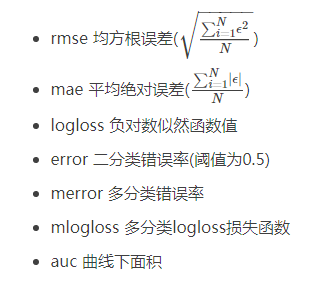

3，Xgboost基本方法和默认参数

xgboost.train(params,dtrain,num_boost_round=10,evals(),obj=None,

feval=None,maximize=False,early_stopping_rounds=None,evals_result=None,

verbose_eval=True,learning_rates=None,xgb_model=None)

　　parms：这是一个字典，里面包含着训练中的参数关键字和对应的值，形式是parms = {'booster':'gbtree','eta':0.1}

　　dtrain：训练的数据

　　num_boost_round：这是指提升迭代的个数

　　evals：这是一个列表，用于对训练过程中进行评估列表中的元素。形式是evals = [(dtrain,'train'),(dval,'val')] 或者是 evals =[(dtrain,'train')] ，对于第一种情况，它使得我们可以在训练过程中观察验证集的效果。

　　obj ：自定义目的函数

　　feval：自定义评估函数

　　maximize：是否对评估函数进行最大化

　　early_stopping_rounds：早起停止次数，假设为100，验证集的误差迭代到一定程度在100次内不能再继续降低，就停止迭代。这要求evals里至少有一个元素，如果有多个，按照最后一个去执行。返回的是最后的迭代次数（不是最好的）。如果early_stopping_rounds存在，则模型会生成三个属性，bst.best_score ,bst.best_iteration和bst.best_ntree_limit

　　evals_result：字典，存储在watchlist中的元素的评估结果

　　verbose_eval（可以输入布尔型或者数值型）：也要求evals里至少有一个元素，如果为True，则对evals中元素的评估结果会输出在结果中；如果输入数字，假设为5，则每隔5个迭代输出一次。

　　learning_rates：每一次提升的学习率的列表

　　xgb_model：在训练之前用于加载的xgb_model

4，模型训练

　　有了参数列表和数据就可以训练模型了

num_round = 10

bst = xgb.train( plst, dtrain, num_round, evallist )

5，模型预测

# X_test类型可以是二维List，也可以是numpy的数组

dtest = DMatrix(X_test)

ans = model.predict(dtest)

　　完整代码如下：

xgb_model.get_booster().save_model('xgb.model')

tar = xgb.Booster(model_file='xgb.model')

x_test = xgb.DMatrix(x_test)

pre=tar.predict(x_test)

act=y_test

print(mean_squared_error(act, pre))

6，保存模型

　　在训练完成之后可以将模型保存下来，也可以查看模型内部的结构

bst.save_model('test.model')

　　导出模型和特征映射（Map）

　　你可以导出模型到txt文件并浏览模型的含义：

# 导出模型到文件

bst.dump_model('dump.raw.txt')

# 导出模型和特征映射

bst.dump_model('dump.raw.txt','featmap.txt')

7，加载模型

　　通过如下方式可以加载模型

bst = xgb.Booster({'nthread':4}) # init model

bst.load_model("model.bin")      # load data

Xgboost实战

　　Xgboost有两大类接口：Xgboost原生接口和sklearn接口，并且Xgboost能够实现分类回归两种任务。下面对这四种情况做以解析。

1，基于Xgboost原生接口的分类

from sklearn.datasets import load_iris

import xgboost as xgb

from xgboost import plot_importance

import matplotlib.pyplot  as plt

from sklearn.model_selection import train_test_split

from sklearn.metrics import accuracy_score  # 准确率
# 记载样本数据集

iris = load_iris()

X,y = iris.data,iris.target

# 数据集分割

X_train,X_test,y_train,y_test = train_test_split(X,y,test_size=0.2,random_state=123457)
# 算法参数

params = {

    'booster':'gbtree',

    'objective':'multi:softmax',

    'num_class':3,

    'gamma':0.1,

    'max_depth':6,

    'lambda':2,

    'subsample':0.7,

    'colsample_bytree':0.7,

    'min_child_weight':3,

    'slient':1,

    'eta':0.1,

    'seed':1000,

    'nthread':4,

}
plst = params.items()
# 生成数据集格式

dtrain = xgb.DMatrix(X_train,y_train)

num_rounds = 500

# xgboost模型训练

model = xgb.train(plst,dtrain,num_rounds)
# 对测试集进行预测

dtest = xgb.DMatrix(X_test)

y_pred = model.predict(dtest)
# 计算准确率

accuracy = accuracy_score(y_test,y_pred)

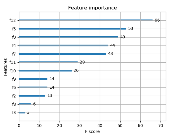
print('accuarcy:%.2f%%'%(accuracy*100))
# 显示重要特征

plot_importance(model)

plt.show()

　　输出预测正确率以及特征重要性：

accuarcy:93.33%

2，基于Xgboost原生接口的回归

import xgboost as xgb

from xgboost import plot_importance

from matplotlib import pyplot as plt

from sklearn.model_selection import train_test_split

from sklearn.datasets import load_boston

from sklearn.metrics import mean_squared_error
# 加载数据集,此数据集时做回归的

boston = load_boston()

X,y = boston.data,boston.target
# Xgboost训练过程

X_train,X_test,y_train,y_test = train_test_split(X,y,test_size=0.2,random_state=0)
# 算法参数

params = {

    'booster':'gbtree',

    'objective':'reg:gamma',

    'gamma':0.1,

    'max_depth':5,

    'lambda':3,

    'subsample':0.7,

    'colsample_bytree':0.7,

    'min_child_weight':3,

    'slient':1,

    'eta':0.1,

    'seed':1000,

    'nthread':4,

}
dtrain = xgb.DMatrix(X_train,y_train)

num_rounds = 300

plst = params.items()

model = xgb.train(plst,dtrain,num_rounds)
# 对测试集进行预测

dtest = xgb.DMatrix(X_test)

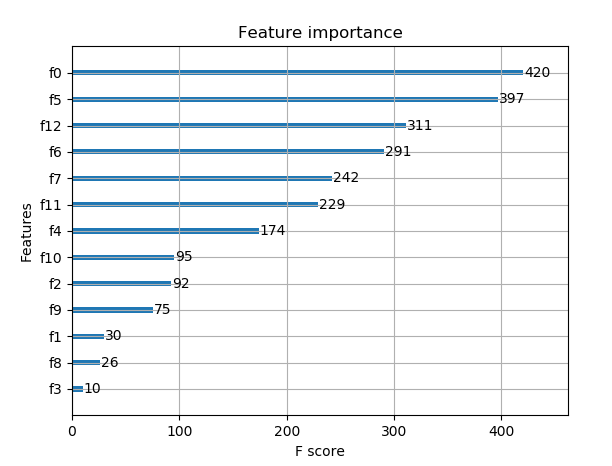
ans = model.predict(dtest)
# 显示重要特征

plot_importance(model)

plt.show()

　　重要特征（值越大，说明该特征越重要）显示结果：

3，Xgboost使用sklearn接口的分类（推荐）

XGBClassifier

from xgboost.sklearn import XGBClassifier
clf = XGBClassifier(

    silent=0,  # 设置成1则没有运行信息输出，最好是设置为0，是否在运行升级时打印消息

    # nthread = 4  # CPU 线程数 默认最大

    learning_rate=0.3 , # 如同学习率

    min_child_weight = 1,

    # 这个参数默认为1，是每个叶子里面h的和至少是多少，对正负样本不均衡时的0-1分类而言

    # 假设h在0.01附近，min_child_weight为1 意味着叶子节点中最少需要包含100个样本

    # 这个参数非常影响结果，控制叶子节点中二阶导的和的最小值，该参数值越小，越容易过拟合

    max_depth=6, # 构建树的深度，越大越容易过拟合

    gamma = 0,# 树的叶子节点上做进一步分区所需的最小损失减少，越大越保守，一般0.1 0.2这样子

    subsample=1, # 随机采样训练样本，训练实例的子采样比

    max_delta_step=0,  # 最大增量步长，我们允许每个树的权重估计

    colsample_bytree=1, # 生成树时进行的列采样

    reg_lambda=1, #控制模型复杂度的权重值的L2正则化项参数，参数越大，模型越不容易过拟合

    # reg_alpha=0, # L1正则项参数

    # scale_pos_weight =1 # 如果取值大于0的话，在类别样本不平衡的情况下有助于快速收敛，平衡正负权重

    # objective = 'multi:softmax', # 多分类问题，指定学习任务和响应的学习目标

    # num_class = 10,  # 类别数，多分类与multisoftmax并用

    n_estimators=100,  # 树的个数

    seed = 1000,  # 随机种子

    # eval_metric ='auc'

)

基于Sckit-learn接口的分类

from sklearn.datasets import load_iris

import xgboost as xgb

from xgboost import plot_importance

from matplotlib import pyplot as plt

from sklearn.model_selection import train_test_split

from sklearn.metrics import accuracy_score
# 加载样本数据集

iris = load_iris()

X,y = iris.data,iris.target

X_train,X_test,y_train,y_test = train_test_split(X,y,test_size=0.2,random_state=12343)
# 训练模型

model = xgb.XGBClassifier(max_depth=5,learning_rate=0.1,n_estimators=160,silent=True,objective='multi:softmax')

model.fit(X_train,y_train)
# 对测试集进行预测

y_pred = model.predict(X_test)
#计算准确率

accuracy = accuracy_score(y_test,y_pred)

print('accuracy:%2.f%%'%(accuracy*100))
# 显示重要特征

plot_importance(model)

plt.show()

　　输出结果：

accuracy:93%

4，基于Scikit-learn接口的回归

import xgboost as xgb

from xgboost import plot_importance

from matplotlib import pyplot as plt

from sklearn.model_selection import train_test_split

from sklearn.datasets import load_boston
# 导入数据集

boston = load_boston()

X ,y = boston.data,boston.target
# Xgboost训练过程

X_train,X_test,y_train,y_test = train_test_split(X,y,test_size=0.2,random_state=0)
model = xgb.XGBRegressor(max_depth=5,learning_rate=0.1,n_estimators=160,silent=True,objective='reg:gamma')

model.fit(X_train,y_train)
# 对测试集进行预测

ans = model.predict(X_test)
# 显示重要特征

plot_importance(model)

plt.show()

5，整理代码1（原生XGB）

from sklearn.model_selection import train_test_split

from sklearn import metrics

from  sklearn.datasets  import  make_hastie_10_2

import xgboost as xgb

#记录程序运行时间

import time

start_time = time.time()

X, y = make_hastie_10_2(random_state=0)

X_train, X_test, y_train, y_test = train_test_split(X, y, test_size=0.5, random_state=0)##test_size测试集合所占比例

#xgb矩阵赋值

xgb_train = xgb.DMatrix(X_train, label=y_train)

xgb_test = xgb.DMatrix(X_test,label=y_test)

##参数

params={

'booster':'gbtree',

'silent':1 ,#设置成1则没有运行信息输出，最好是设置为0.

#'nthread':7,# cpu 线程数 默认最大

'eta': 0.007, # 如同学习率

'min_child_weight':3,

# 这个参数默认是 1，是每个叶子里面 h 的和至少是多少，对正负样本不均衡时的 0-1 分类而言

#，假设 h 在 0.01 附近，min_child_weight 为 1 意味着叶子节点中最少需要包含 100 个样本。

#这个参数非常影响结果，控制叶子节点中二阶导的和的最小值，该参数值越小，越容易 overfitting。

'max_depth':6, # 构建树的深度，越大越容易过拟合

'gamma':0.1,  # 树的叶子节点上作进一步分区所需的最小损失减少,越大越保守，一般0.1、0.2这样子。

'subsample':0.7, # 随机采样训练样本

'colsample_bytree':0.7, # 生成树时进行的列采样

'lambda':2,  # 控制模型复杂度的权重值的L2正则化项参数，参数越大，模型越不容易过拟合。

#'alpha':0, # L1 正则项参数

#'scale_pos_weight':1, #如果取值大于0的话，在类别样本不平衡的情况下有助于快速收敛。

#'objective': 'multi:softmax', #多分类的问题

#'num_class':10, # 类别数，多分类与 multisoftmax 并用

'seed':1000, #随机种子

#'eval_metric': 'auc'

}

plst = list(params.items())

num_rounds = 100 # 迭代次数

watchlist = [(xgb_train, 'train'),(xgb_test, 'val')]
#训练模型并保存

# early_stopping_rounds 当设置的迭代次数较大时，early_stopping_rounds 可在一定的迭代次数内准确率没有提升就停止训练

model = xgb.train(plst, xgb_train, num_rounds, watchlist,early_stopping_rounds=100,pred_margin=1)

#model.save_model('./model/xgb.model') # 用于存储训练出的模型

print "best best_ntree_limit",model.best_ntree_limit

y_pred = model.predict(xgb_test,ntree_limit=model.best_ntree_limit)

print ('error=%f' % (  sum(1 for i in range(len(y_pred)) if int(y_pred[i]>0.5)!=y_test[i]) /float(len(y_pred))))

#输出运行时长

cost_time = time.time()-start_time

print "xgboost success!",'\n',"cost time:",cost_time,"(s)......"

6，整理代码2（XGB使用sklearn）

from sklearn.model_selection import train_test_split

from sklearn import metrics

from  sklearn.datasets  import  make_hastie_10_2

from xgboost.sklearn import XGBClassifier

X, y = make_hastie_10_2(random_state=0)

X_train, X_test, y_train, y_test = train_test_split(X, y, test_size=0.5, random_state=0)##test_size测试集合所占比例

clf = XGBClassifier(

silent=0 ,#设置成1则没有运行信息输出，最好是设置为0.是否在运行升级时打印消息。

#nthread=4,# cpu 线程数 默认最大

learning_rate= 0.3, # 如同学习率

min_child_weight=1,

# 这个参数默认是 1，是每个叶子里面 h 的和至少是多少，对正负样本不均衡时的 0-1 分类而言

#，假设 h 在 0.01 附近，min_child_weight 为 1 意味着叶子节点中最少需要包含 100 个样本。

#这个参数非常影响结果，控制叶子节点中二阶导的和的最小值，该参数值越小，越容易 overfitting。

max_depth=6, # 构建树的深度，越大越容易过拟合

gamma=0,  # 树的叶子节点上作进一步分区所需的最小损失减少,越大越保守，一般0.1、0.2这样子。

subsample=1, # 随机采样训练样本 训练实例的子采样比

max_delta_step=0,#最大增量步长，我们允许每个树的权重估计。

colsample_bytree=1, # 生成树时进行的列采样

reg_lambda=1,  # 控制模型复杂度的权重值的L2正则化项参数，参数越大，模型越不容易过拟合。

#reg_alpha=0, # L1 正则项参数

#scale_pos_weight=1, #如果取值大于0的话，在类别样本不平衡的情况下有助于快速收敛。平衡正负权重

#objective= 'multi:softmax', #多分类的问题 指定学习任务和相应的学习目标

#num_class=10, # 类别数，多分类与 multisoftmax 并用

n_estimators=100, #树的个数

seed=1000 #随机种子

#eval_metric= 'auc'

)

clf.fit(X_train,y_train,eval_metric='auc')

#设置验证集合 verbose=False不打印过程

clf.fit(X_train, y_train,eval_set=[(X_train, y_train), (X_val, y_val)],eval_metric='auc',verbose=False)

#获取验证集合结果

evals_result = clf.evals_result()

y_true, y_pred = y_test, clf.predict(X_test)

print"Accuracy : %.4g" % metrics.accuracy_score(y_true, y_pred)

#回归

#m_regress = xgb.XGBRegressor(n_estimators=1000,seed=0)

Xgboost参数调优的一般方法

调参步骤：

　　1，选择较高的学习速率（learning rate）。一般情况下，学习速率的值为0.1.但是，对于不同的问题，理想的学习速率有时候会在0.05~0.3之间波动。选择对应于此学习速率的理想决策树数量。Xgboost有一个很有用的函数“cv”，这个函数可以在每一次迭代中使用交叉验证，并返回理想的决策树数量。

　　2，对于给定的学习速率和决策树数量，进行决策树特定参数调优（max_depth , min_child_weight , gamma , subsample,colsample_bytree）在确定一棵树的过程中，我们可以选择不同的参数。

　　3，Xgboost的正则化参数的调优。（lambda , alpha）。这些参数可以降低模型的复杂度，从而提高模型的表现。

　　4，降低学习速率，确定理想参数。

　　下面详细的进行这些操作。

第一步：确定学习速率和tree_based参数调优的估计器数目

　　为了确定Boosting参数，我们要先给其他参数一个初始值。咱们先按照如下方法取值：

1，max_depth = 5：这个参数的取值最好在3-10之间，我选的起始值为5，但是你可以选择其他的值。起始值在4-6之间都是不错的选择。
2，min_child_weight = 1 ：这里选择了一个比较小的值，因为这是一个极不平衡的分类问题。因此，某些叶子节点下的值会比较小。
3，gamma = 0 :起始值也可以选择其它比较小的值，在0.1到0.2之间就可以，这个参数后继也是要调整的。
4，subsample,colsample_bytree = 0.8 这个是最常见的初始值了。典型值的范围在0.5-0.9之间。
5，scale_pos_weight =1 这个值时因为类别十分不平衡。

　　注意，上面这些参数的值知识一个初始的估计值，后继需要调优。这里把学习速率就设成默认的0.1。然后用Xgboost中的cv函数来确定最佳的决策树数量。

from xgboost import XGBClassifier

xgb1 = XGBClassifier(

 learning_rate =0.1,

 n_estimators=1000,

 max_depth=5,

 min_child_weight=1,

 gamma=0,

 subsample=0.8,

 colsample_bytree=0.8,

 objective= 'binary:logistic',

 nthread=4,

 scale_pos_weight=1,

 seed=27)

第二步：max_depth和min_weight参数调优

　　我们先对这两个参数调优，是因为他们对最终结果有很大的影响。首先，我们先大范围地粗略参数，然后再小范围的微调。

　　注意：在这一节我会进行高负荷的栅格搜索（grid search），这个过程大约需要15-30分钟甚至更久，具体取决于你系统的性能，你也可以根据自己系统的性能选择不同的值。

　　网格搜索scoring = 'roc_auc' 只支持二分类，多分类需要修改scoring（默认支持多分类）

param_test1 = {

 'max_depth':range(3,10,2),

 'min_child_weight':range(1,6,2)

}

#param_test2 = {

 'max_depth':[4,5,6],

 'min_child_weight':[4,5,6]

}

from sklearn import svm, grid_search, datasets

from sklearn import grid_search

gsearch1 = grid_search.GridSearchCV(

estimator = XGBClassifier(

learning_rate =0.1,

n_estimators=140, max_depth=5,

min_child_weight=1,

gamma=0,

subsample=0.8,

colsample_bytree=0.8,

objective= 'binary:logistic',

nthread=4,

scale_pos_weight=1,

seed=27),

param_grid = param_test1,

scoring='roc_auc',

n_jobs=4,

iid=False,

cv=5)

gsearch1.fit(train[predictors],train[target])

gsearch1.grid_scores_, gsearch1.best_params_,gsearch1.best_score_

#网格搜索scoring='roc_auc'只支持二分类，多分类需要修改scoring(默认支持多分类)

第三步：gamma参数调优

　　在已经调整好其他参数的基础上，我们可以进行gamma参数的调优了。Gamma参数取值范围很大，这里我们设置为5，其实你也可以取更精确的gamma值。

param_test3 = {

 'gamma':[i/10.0 for i in range(0,5)]

}
gsearch3 = GridSearchCV(estimator = XGBClassifier( learning_rate =0.1,

 n_estimators=140, max_depth=4,min_child_weight=6, gamma=0,

subsample=0.8, colsample_bytree=0.8,objective= 'binary:logistic',

nthread=4, scale_pos_weight=1,seed=27),  param_grid = param_test3, scoring='roc_auc',n_jobs=4,iid=False, cv=5)
gsearch3.fit(train[predictors],train[target])
gsearch3.grid_scores_, gsearch3.best_params_, gsearch3.best_score_

param_test3 = {

 'gamma':[i/10.0 for i in range(0,5)]

}

gsearch3 = GridSearchCV(

estimator = XGBClassifier(

learning_rate =0.1,

n_estimators=140,

max_depth=4,

min_child_weight=6,

gamma=0,

subsample=0.8,

colsample_bytree=0.8,

objective= 'binary:logistic',

nthread=4,

scale_pos_weight=1,

seed=27),

param_grid = param_test3,

scoring='roc_auc',

n_jobs=4,

iid=False,

cv=5)

gsearch3.fit(train[predictors],train[target])

gsearch3.grid_scores_, gsearch3.best_params_, gsearch3.best_score_

第四步：调整subsample 和 colsample_bytree参数

　　尝试不同的subsample 和 colsample_bytree 参数。我们分两个阶段来进行这个步骤。这两个步骤都取0.6,0.7,0.8,0.9作为起始值。

#取0.6,0.7,0.8,0.9作为起始值

param_test4 = {

 'subsample':[i/10.0 for i in range(6,10)],

 'colsample_bytree':[i/10.0 for i in range(6,10)]

}
gsearch4 = GridSearchCV(

estimator = XGBClassifier(

learning_rate =0.1,

n_estimators=177,

max_depth=3,

min_child_weight=4,

gamma=0.1,

subsample=0.8,

colsample_bytree=0.8,

objective= 'binary:logistic',

nthread=4,

scale_pos_weight=1,

seed=27),

param_grid = param_test4,

scoring='roc_auc',

n_jobs=4,

iid=False,

cv=5)

gsearch4.fit(train[predictors],train[target])

gsearch4.grid_scores_, gsearch4.best_params_, gsearch4.best_score_

第五步：正则化参数调优

　　由于gamma函数提供了一种更加有效的降低过拟合的方法，大部分人很少会用到这个参数，但是我们可以尝试用一下这个参数。

param_test6 = {

 'reg_alpha':[1e-5, 1e-2, 0.1, 1, 100]

}

gsearch6 = GridSearchCV(

estimator = XGBClassifier(

learning_rate =0.1,

n_estimators=177,

max_depth=4,

min_child_weight=6,

gamma=0.1,

subsample=0.8,

colsample_bytree=0.8,

objective= 'binary:logistic',

nthread=4,

scale_pos_weight=1,

seed=27),

param_grid = param_test6,

scoring='roc_auc',

n_jobs=4,

iid=False,

cv=5)

gsearch6.fit(train[predictors],train[target])

gsearch6.grid_scores_, gsearch6.best_params_, gsearch6.best_score_

第六步：降低学习速率

　　最后，我们使用较低的学习速率，以及使用更多的决策树，我们可以用Xgboost中CV函数来进行这一步工作。

xgb4 = XGBClassifier(

 learning_rate =0.01,

 n_estimators=5000,

 max_depth=4,

 min_child_weight=6,

 gamma=0,

 subsample=0.8,

 colsample_bytree=0.8,

 reg_alpha=0.005,

 objective= 'binary:logistic',

 nthread=4,

 scale_pos_weight=1,

 seed=27)

modelfit(xgb4, train, predictors)

　　总结一下，要想模型的表现有大幅的提升，调整每个参数带来的影响也必须清楚，仅仅靠着参数的调整和模型的小幅优化，想要让模型的表现有个大幅度提升是不可能的。要想模型的表现有质的飞跃，需要依靠其他的手段。诸如，特征工程(feature egineering) ，模型组合(ensemble of model),以及堆叠(stacking)等。

第七步：Python示例

import xgboost as xgb

import pandas as pd

#获取数据

from sklearn import cross_validation

from sklearn.datasets import load_iris

iris = load_iris()

#切分数据集

X_train, X_test, y_train, y_test = cross_validation.train_test_split(iris.data, iris.target, test_size=0.33, random_state=42)

#设置参数

m_class = xgb.XGBClassifier(

 learning_rate =0.1,

 n_estimators=1000,

 max_depth=5,

 gamma=0,

 subsample=0.8,

 colsample_bytree=0.8,

 objective= 'binary:logistic',

 nthread=4,

 seed=27)

#训练

m_class.fit(X_train, y_train)

test_21 = m_class.predict(X_test)

print "Accuracy : %.2f" % metrics.accuracy_score(y_test, test_21)

#预测概率

#test_2 = m_class.predict_proba(X_test)

#查看AUC评价标准

from sklearn import metrics

print "Accuracy : %.2f" % metrics.accuracy_score(y_test, test_21)

##必须二分类才能计算

##print "AUC Score (Train): %f" % metrics.roc_auc_score(y_test, test_2)

#查看重要程度

feat_imp = pd.Series(m_class.booster().get_fscore()).sort_values(ascending=False)

feat_imp.plot(kind='bar', title='Feature Importances')

import matplotlib.pyplot as plt

plt.show()

#回归

#m_regress = xgb.XGBRegressor(n_estimators=1000,seed=0)

#m_regress.fit(X_train, y_train)

#test_1 = m_regress.predict(X_test)

XGBoost输出特征重要性以及筛选特征

1，梯度提升算法是如何计算特征重要性的？

　　使用梯度提升算法的好处是在提升树被创建后，可以相对直接地得到每个属性的重要性得分。一般来说，重要性分数，衡量了特征在模型中的提升决策树构建中的价值。一个属性越多的被用来在模型中构建决策树，它的重要性就相对越高。

　　属性重要性是通过对数据集中的每个属性进行计算，并进行排序得到。在单个决策树中通过每个属性分裂点改进性能度量的量来计算属性重要性。由节点负责加权和记录次数，也就是说一个属性对分裂点改进性能度量越大（越靠近根节点），权值越大；被越多提升树所选择，属性越重要。性能度量可以是选择分裂节点的Gini纯度，也可以是其他度量函数。

　　最终将一个属性在所有提升树中的结果进行加权求和后然后平均，得到重要性得分。

2，绘制特征重要性

　　一个已训练的Xgboost模型能够自动计算特征重要性，这些重要性得分可以通过成员变量feature_importances_得到。可以通过如下命令打印：

print(model.feature_importances_)

　　我们可以直接在条形图上绘制这些分数，以便获得数据集中每个特征的相对重要性的直观显示，例如：

# plot

pyplot.bar(range(len(model.feature_importances_)), model.feature_importances_)

pyplot.show()

　　我们可以通过在the Pima Indians onset of diabetes 数据集上训练XGBoost模型来演示，并从计算的特征重要性中绘制条形图。

# plot feature importance manually

from numpy import loadtxt

from xgboost import XGBClassifier

from matplotlib import pyplot

from sklearn.datasets import load_iris

# load data

dataset = load_iris()

# split data into X and y

X = dataset.data

y = dataset.target

# fit model no training data

model = XGBClassifier()

model.fit(X, y)

# feature importance

print(model.feature_importances_)

# plot

pyplot.bar(range(len(model.feature_importances_)), model.feature_importances_)

pyplot.show()

　　运行这个实例，首先输出特征重要性分数：

[0.17941953 0.11345647 0.41556728 0.29155672]

　　相对重要性条形图：

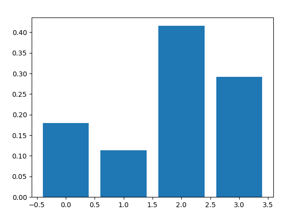
　　这种绘制的缺点在于，只显示了特征重要性而没有排序，可以在绘制之前对特征重要性得分进行排序。

　　通过内建的绘制函数进行特征重要性得分排序后的绘制，这个函数就是plot_importance()，示例如下：

# plot feature importance manually

from numpy import loadtxt

from xgboost import XGBClassifier

from matplotlib import pyplot

from sklearn.datasets import load_iris

from xgboost import plot_importance
# load data

dataset = load_iris()

# split data into X and y

X = dataset.data

y = dataset.target

# fit model no training data

model = XGBClassifier()

model.fit(X, y)

# feature importance

print(model.feature_importances_)

# plot feature importance
plot_importance(model)

pyplot.show()

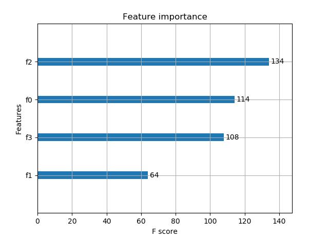
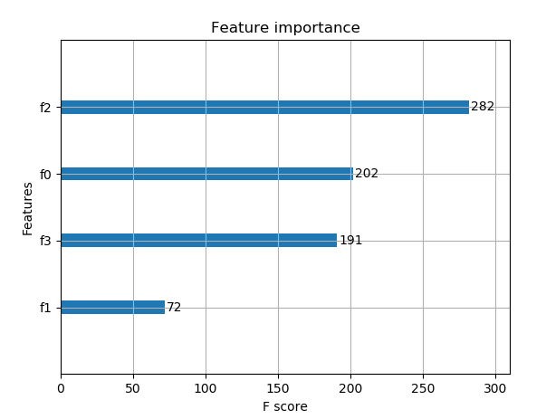
　　示例得到条形图：

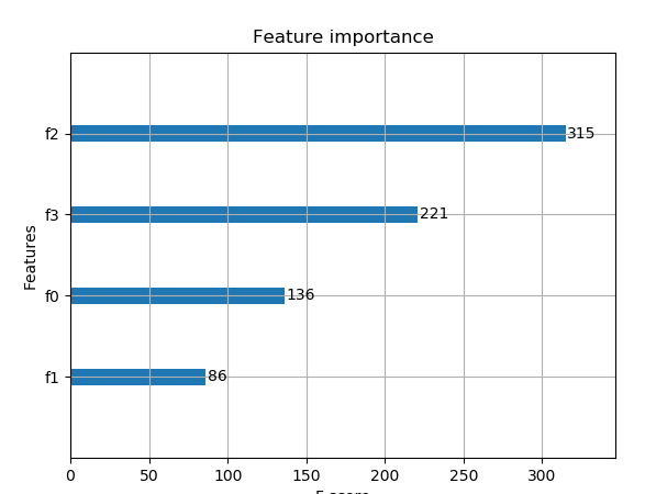
　　根据其在输入数组的索引，特征被自动命名为f0~f3，在问题描述中手动的将这些索引映射到名称，我们可以看到，f2具有最高的重要性，f1具有最低的重要性。

3，根据Xgboost特征重要性得分进行特征选择

　　特征重要性得分，可以用于在scikit-learn中进行特征选择。通过SelectFromModel类实现，该类采用模型并将数据集转换为具有选定特征的子集。这个类可以采取预先训练的模型，例如在整个数据集上训练的模型。然后，它可以阈值来决定选择哪些特征。当在SelectFromModel实例上调用transform()方法时，该阈值被用于在训练集和测试集上一致性选择相同特征。

　　在下面的示例中，我们首先在训练集上训练xgboost模型，然后在测试上评估。使用从训练数据集计算的特征重要性，然后，将模型封装在一个SelectFromModel实例中。我们使用这个来选择训练集上的特征，用所选择的特征子集训练模型，然后在相同的特征方案下对测试集进行评估。

# select features using threshold

selection = SelectFromModel(model, threshold=thresh, prefit=True)

select_X_train = selection.transform(X_train)

# train model

selection_model = XGBClassifier()

selection_model.fit(select_X_train, y_train)

# eval model

select_X_test = selection.transform(X_test)

y_pred = selection_model.predict(select_X_test)

　　我们可以通过测试多个阈值，来从特征重要性中选择特征。具体而言，每个输入变量的特征重要性，本质上允许我们通过重要性来测试每个特征子集。

完整代码如下：

# plot feature importance manually

import numpy as np

from xgboost import XGBClassifier

from matplotlib import pyplot

from sklearn.datasets import load_iris

from xgboost import plot_importance

from sklearn.model_selection import train_test_split

from sklearn.metrics import accuracy_score

from sklearn.feature_selection import SelectFromModel
# load data

dataset = load_iris()

# split data into X and y

X = dataset.data

y = dataset.target
# split data into train and test sets

X_train,X_test,y_train,y_test = train_test_split(X,y,test_size=0.33,random_state=7)
# fit model no training data

model = XGBClassifier()

model.fit(X_train, y_train)

# feature importance

print(model.feature_importances_)
# make predictions for test data and evaluate

y_pred = model.predict(X_test)

predictions = [round(value) for value in y_pred]

accuracy = accuracy_score(y_test,predictions)

print("Accuracy:%.2f%%"%(accuracy*100.0))
#fit model using each importance as a threshold

thresholds = np.sort(model.feature_importances_)

for thresh in thresholds:

    # select features using threshold

    selection = SelectFromModel(model,threshold=thresh,prefit=True )

    select_X_train = selection.transform(X_train)

    # train model

    selection_model = XGBClassifier()

    selection_model.fit(select_X_train, y_train)

    # eval model

    select_X_test = selection.transform(X_test)

    y_pred = selection_model.predict(select_X_test)

    predictions = [round(value) for value in y_pred]

    accuracy = accuracy_score(y_test,predictions)

    print("Thresh=%.3f, n=%d, Accuracy: %.2f%%" % (thresh, select_X_train.shape[1], accuracy * 100.0))

　　运行示例，得到输出：

[0.20993228 0.09029345 0.54176074 0.15801354]

Accuracy:92.00%

Thresh=0.090, n=4, Accuracy: 92.00%

Thresh=0.158, n=3, Accuracy: 92.00%

Thresh=0.210, n=2, Accuracy: 86.00%

Thresh=0.542, n=1, Accuracy: 90.00%

　　我们可以看到，模型的性能通常随着所选择的特征的数量减少，在这一问题上，可以对测试集准确率和模型复杂度做一个权衡，例如选择三个特征，接受准确率为92%，这可能是对这样一个小数据集的清洗，但是对于更大的数据集和使用交叉验证作为模型评估方案可能是更有用的策略。

4，网格搜索

代码1：

from sklearn.model_selection import GridSearchCV

tuned_parameters= [{'n_estimators':[100,200,500],

                  'max_depth':[3,5,7], ##range(3,10,2)

                  'learning_rate':[0.5, 1.0],

                  'subsample':[0.75,0.8,0.85,0.9]

                  }]

tuned_parameters= [{'n_estimators':[100,200,500,1000]

                  }]

clf = GridSearchCV(XGBClassifier(silent=0,nthread=4,learning_rate= 0.5,min_child_weight=1, max_depth=3,gamma=0,subsample=1,colsample_bytree=1,reg_lambda=1,seed=1000), param_grid=tuned_parameters,scoring='roc_auc',n_jobs=4,iid=False,cv=5)

clf.fit(X_train, y_train)

##clf.grid_scores_, clf.best_params_, clf.best_score_

print(clf.best_params_)

y_true, y_pred = y_test, clf.predict(X_test)

print"Accuracy : %.4g" % metrics.accuracy_score(y_true, y_pred)

y_proba=clf.predict_proba(X_test)[:,1]

print "AUC Score (Train): %f" % metrics.roc_auc_score(y_true, y_proba)

代码2：

from sklearn.model_selection import GridSearchCV

parameters= [{'learning_rate':[0.01,0.1,0.3],'n_estimators':[1000,1200,1500,2000,2500]}]

clf = GridSearchCV(XGBClassifier(

             max_depth=3,

             min_child_weight=1,

             gamma=0.5,

             subsample=0.6,

             colsample_bytree=0.6,

             objective= 'binary:logistic', #逻辑回归损失函数

             scale_pos_weight=1,

             reg_alpha=0,

             reg_lambda=1,

             seed=27

            ),

            param_grid=parameters,scoring='roc_auc')

clf.fit(X_train, y_train)

print(clf.best_params_)

y_pre= clf.predict(X_test)

y_pro= clf.predict_proba(X_test)[:,1]

print "AUC Score : %f" % metrics.roc_auc_score(y_test, y_pro)

print"Accuracy : %.4g" % metrics.accuracy_score(y_test, y_pre)

输出特征重要性：

import pandas as pd

import matplotlib.pylab as plt

feat_imp = pd.Series(clf.booster().get_fscore()).sort_values(ascending=False)

feat_imp.plot(kind='bar', title='Feature Importances')

plt.ylabel('Feature Importance Score')

plt.show()

补充：关于随机种子——random_state

　　random_state是一个随机种子，是在任意带有随机性的类或者函数里作为参数来控制随机模式。random_state取某一个值的时候，也就确定了一种规则。

　　random_state可以用于很多函数，比如训练集测试集的划分；构建决策树；构建随机森林

1，划分训练集和测试集的类train_test_split

　　随机数种子控制每次划分训练集和测试集的模式，其取值不变时划分得到的结果一模一样，其值改变时，划分得到的结果不同。若不设置此参数，则函数会自动选择一种随机模式，得到的结果也就不同。

2，构建决策树的函数

clf = tree.DecisionTreeClassifier(criterion="entropy",random_state=30,splitter="random")

　　其取值不变时，用相同的训练集建树得到的结果一模一样，对测试集的预测结果也是一样的

　　其取值改变时，得到的结果不同；

　　若不设置此参数，则函数会自动选择一种随机模式，每次得到的结果也就不同。

3，构建随机森林

clf = RandomForestClassifier(random_state=0)

　　其取值不变时，用相同的训练集建树得到的结果一模一样，对测试集的预测结果也是一样的

　　其取值改变时，得到的结果不同；

　　若不设置此参数，则函数会自动选择一种随机模式，每次得到的结果也就不同。

4，总结

　　在需要设置random_state的地方给其赋值，当多次运行此段代码得到完全一样的结果，别人运行代码也可以复现你的过程。若不设置此参数则会随机选择一个种子，执行结果也会因此不同。虽然可以对random_state进行调参，但是调参后再训练集上表现好的模型未必在陌生训练集上表现好，所以一般会随便选择一个random_state的值作为参数。

　　对于那些本质上是随机的过程，我们有必要控制随机的状态，这样才能重复的展现相同的结果。如果对随机状态不加控制，那么实验的结果就无法固定，而是随机的显示。

参考文献：

https://blog.csdn.net/waitingzby/article/details/81610495

https://blog.csdn.net/u011089523/article/details/72812019

https://blog.csdn.net/luanpeng825485697/article/details/79907149

https://xgboost.readthedocs.io/en/latest/parameter.html#general-parameters

上一篇： Python基础三. 函数、lambda、filter、map、reduce
下一篇： python获取ESTABLISHED

Python机器学习笔记：XgBoost算法

前言

1，Xgboost简介

2，Xgboost的优点

2.1 正则化

2.2 并行处理

2.3 灵活性

2.4 缺失值处理

2.5 剪枝

2.6 内置交叉验证

3，Xgboost的离线安装

Xgboost模型详解

1，Xgboost能加载的各种数据格式解析

2，Xgboost的模型参数

2.1， 通用参数

2.2，tree booster参数

2.3，Linear Booster参数

2.4，学习目标参数

3，Xgboost基本方法和默认参数

4，模型训练

5，模型预测

6，保存模型

7，加载模型

Xgboost实战

1，基于Xgboost原生接口的分类

2，基于Xgboost原生接口的回归

3，Xgboost使用sklearn接口的分类（推荐）

XGBClassifier

基于Sckit-learn接口的分类

4，基于Scikit-learn接口的回归

5，整理代码1（原生XGB）

6，整理代码2（XGB使用sklearn）

Xgboost参数调优的一般方法

调参步骤：

第一步：确定学习速率和tree_based参数调优的估计器数目

第二步：max_depth和min_weight参数调优

第三步：gamma参数调优

第四步：调整subsample 和 colsample_bytree参数

第五步：正则化参数调优

第六步：降低学习速率

第七步：Python示例

XGBoost输出特征重要性以及筛选特征

1，梯度提升算法是如何计算特征重要性的？

2，绘制特征重要性

3，根据Xgboost特征重要性得分进行特征选择

4，网格搜索

补充：关于随机种子——random_state

1，划分训练集和测试集的类train_test_split

2，构建决策树的函数

3，构建随机森林

4，总结

相关文章

Python基础三. 函数、lambda、filter、map、reduce

python基础学习Day12 生成器

Python基础之变量，常量，注释，数据类型

python获取ESTABLISHED

python绘图增加中文标题

python画箱线图

2.1，通用参数